Problem Statement and Background

In the modern music scene, more and more audio content is accompanied by visual aids. Whether through music videos, album covers, promotional clips, or live lighting and visuals, music and video are closely linked. Despite this, creating videos to accurately match music can often be challenging for musicians. Therefore, musicians may want visuals to accompany the music they create, without having to design these themselves.

Our project aims to match input audio clips to similar video clips stored in a database. With this tool, artists can stitch together visuals from music videos or other visual sources to generate visual accompaniments for their music.

For technical evaluation, we planned to focus on both validation and training accuracy of our network. Although training accuracy is not a good measure of the network’s ability to generalize to other data, it is a helpful informal metric for quickly evaluating the learning power of different network architectures. Validation accuracy is a more accurate measure of the ability to generalize to data that it has never seen before.

We quantitatively use the Recall or Recovery@K metric, a common metric in “cross-modal retrieval” which measures the percentage of queries that recover a correct match in the top K matches. We achieve a 15-20% R@5.

We also planned to evaluate our model’s functionality by performing many real-world tests. The most basic test is to pass in a song as audio input and generate an accompanying music video from our entire video library to judge its efficacy on fitting the style of music. To further explore this, we also generated the three closest and farthest matches for a given audio input.

Related Works

• Content-based Representations of Audio Using Siamese Networks by Manocha et.al. retrieves semantically similar audio recordings given an audio clip input, and architecturally is the model most similar to ours.
• Automatic Music Video Generation Based on Emotion Oriented Pseudo Song Prediction and Matching by Lin et. al. uses a multi-task network to jointly learn the relationship among audio, video, and emotion. They achieve a 76% recovery accuracy, but utilize a much more complicated model.
• Content-Based Video-Music Retrieval Using Soft Intra-Modal Structure Constraint by Hong et. al. is also very similar to ours, and achieves approximately the same recovery rate. Their model uses two separate networks to embed audio and video.

Approach

Data

Our final dataset (and video ‘library’) consists of over 900 music videos downloaded from YouTube using the youtube-dl utility. 200 of these were downloaded from VEVO genre playlists, representing EDM (Electronic Dance Music) and Pop music videos from the last couple months; the other 700 were sourced from a music video dataset . From their 200K video list, we randomly sample approximately 700. This dataset includes videos across all genres, as well as unofficial and parody music videos.

After downloading, we use ffmpeg to split the videos into 10 second video and audio (.mp4 and .wav) clips. Each video/audio clip is labeled with a clip ID (unique) and video ID (shared between all clips of the same video).

We then use two off the shelf feature extractors, YouTube-8M for video features and AudioSet. AudioSet uses a VGG-like architecture as described in Hershey17 and YouTube-8M uses a state of the art Inception network to extract a 128-feature PCA-ed and quantized vector per second. Thus, our model these as input a concatenated, 1280-feature vector for video and audio each.

Model

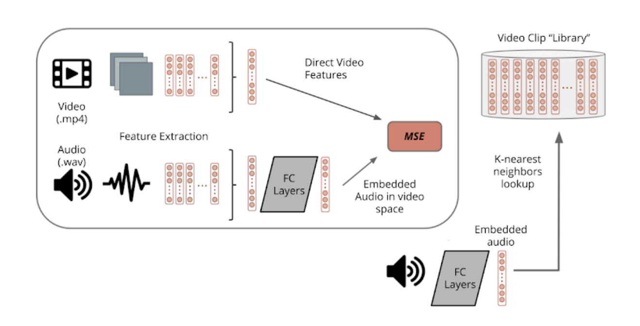
Our baseline model is a single feed-forward network that aims to turn one feature vector (audio) into the other (video, or vice versa). It turns our task into a regression problem, aiming to embed the 1280-feature audio vector into video space by minimizing the MSE, using the video feature vector as ground truth. We use 4 fully connected layers with tanh activations and .3 dropout.

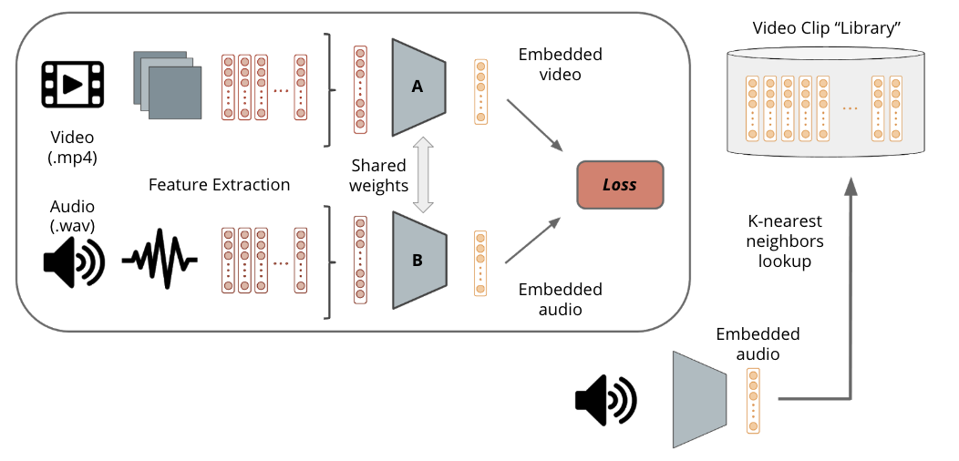
Our final model uses a similiarity siamese network approach, using a similar feed-forward model as a subnetwork. This time, the subnetwork consists of 4 fully-connected layers with dimensions [1024, 256, 128, 128] and .9 dropout. Both audio and video inputs are passed into copies of this subnetwork (sharing weights), and output a 128-feature embedding.

The dual networks are trained with batch size 16, alternating between batches comprised of matching (same clip label on audio and video) and non-matching (different clip label) pairs. We use the ADAM optimizer with a learning rate of .0001 to minimize contrastive loss with L1=.001 and L2=.01 regularizers using some margin m=1 and supervised on the clip label, which aims to embed the video and audio vectors from the same clip into the same representation, and video and audio vectors from different clips into embeddings with at least distance m. We also experimented with supervising by the video label, but mostly just for visualization purposes (more in Results below).

After we have a trained model, we can feed in a set of video clips (either previously seen by the network at training or not) to generate a library of embedded video clip. We can then feed in an audio clip and do a nearest neighbors lookup for the embedded audio. Feeding in audio clips of an entire song allows us to splice together a music video, using clips in our library.

Tools

We use two out of the box feature extractors for audio and video, since we don’t necessarily require any fine-tuning or specific way of features to be extracted; both YouTube-8M and AudioSet are intended for video and audio classification, so the features should be representative enough for our task as well.

youtube-dl and ffmpeg are very useful utilities, though ffmpeg can be quite slow.

Using the siamese network architecture is useful as it requires less data, since the subnetworks share weights. It is also well-suited for learning similarity.

Results

Training & Data Partitioning

We use our 900+ downloaded music video dataset that yields nearly 18,000 audio-video clip pairs. We use an 80:20 training:validation test split and measure accuracy on a R@5 metric and a batch size of 100.

Best Model Results

We present recall accuracy graphs for our best model. These are generated alongside training time, on random validation batches of size 100.

Random	R@1	R@5

R@10	R@25

Discussion

Our initial attempts at training the network had layer dimensions from 1024 to 128, and dropouots set to .3 or .4; this resulted in severe overfitting on training data. The network would reach 100% training accuracy in 2-3 epochs and not learn anything. Part of the motivation to share weights between the subnetworks is to reduce trainable parameters, so we chose to embrace this and drastically reduce the layer dimensions and drastically increase the dropout rates.

Training Loss	Training Accuracy R@5	Validation Accuracy R@5

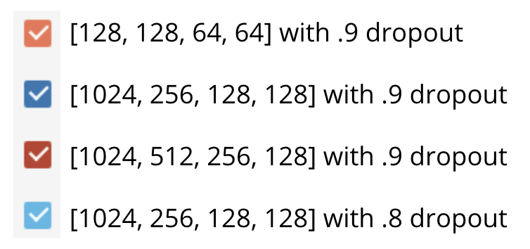Fig 4.

Upon further investigation, we see that the layer dimensions has less effect – our best performing model actually had its initial layer sized at 1024. It was truly the dropout rate that made a bigger difference, which makes sense; .9 is much more aggressive.

We also show the effect of the margin in the contrastive loss:

Training Loss	Training Accuracy R@5	Validation Accuracy R@5

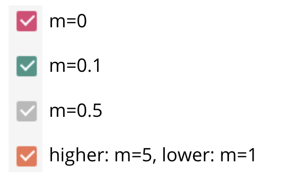Fig 5.

Apologies for the unfortunate use of orange twice :(. Nevertheless, we see that the higher margin values are much more successful.

We saw no improvement for higher margin values such as 6, 8, or 10.

Other Comments

We nearly tripled the size of our dataset and noticed little difference in our results. Moreover, we note that the validation accuracy reaches its max (for that particular set of parameters) within very few epochs.

More Quantitative Results

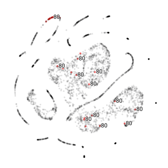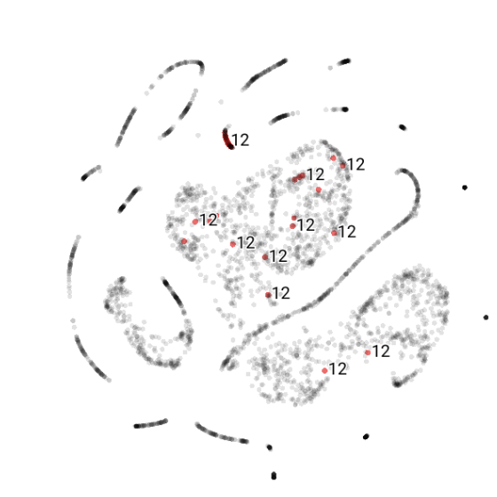
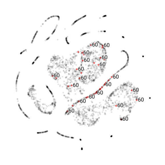
We can see that the model does a decent job at grouping most clips from the same video nearby one another – i.e. embeds clips labeled with the same video ID nearby one another. Video 60’s clips along that trail may suggest some temporal component.

Qualitative Results

We hoped to generate many more qualitative examples, but ran out of time. One example was to demonstrate the variation in generated music videos by taking a limited video library set, and passing in different audio clips.

Another was to take non-music video video content, such as a nature documentary, and see what results could be generated from that.

We may add those results to this page, but note that if they appear, they were added after the deadline.

Lessons Learned

The biggest lesson we learned was that working with the combined audio-video space required for this task is incredibly difficult for two main reasons. First of all, the space’s size makes it incredibly hard to compile a representative dataset. We tried to combat this by focusing our model to specific subsections of the dataset such as the same genre of music or a single video type in the video library.

Secondly, it was very hard to balance the number of parameters in our model. On one hand, we needed a larger amount of parameters to effectively model the space we were targeting. On the other hand, however, our models seemed especially prone to quickly overfitting the training data. To combat this concern, we implemented a very high dropout rate.